Counting Sort
Counting sort sorts by counting the occurrences of elements and is typically applied to integer arrays.
Simple Implementation
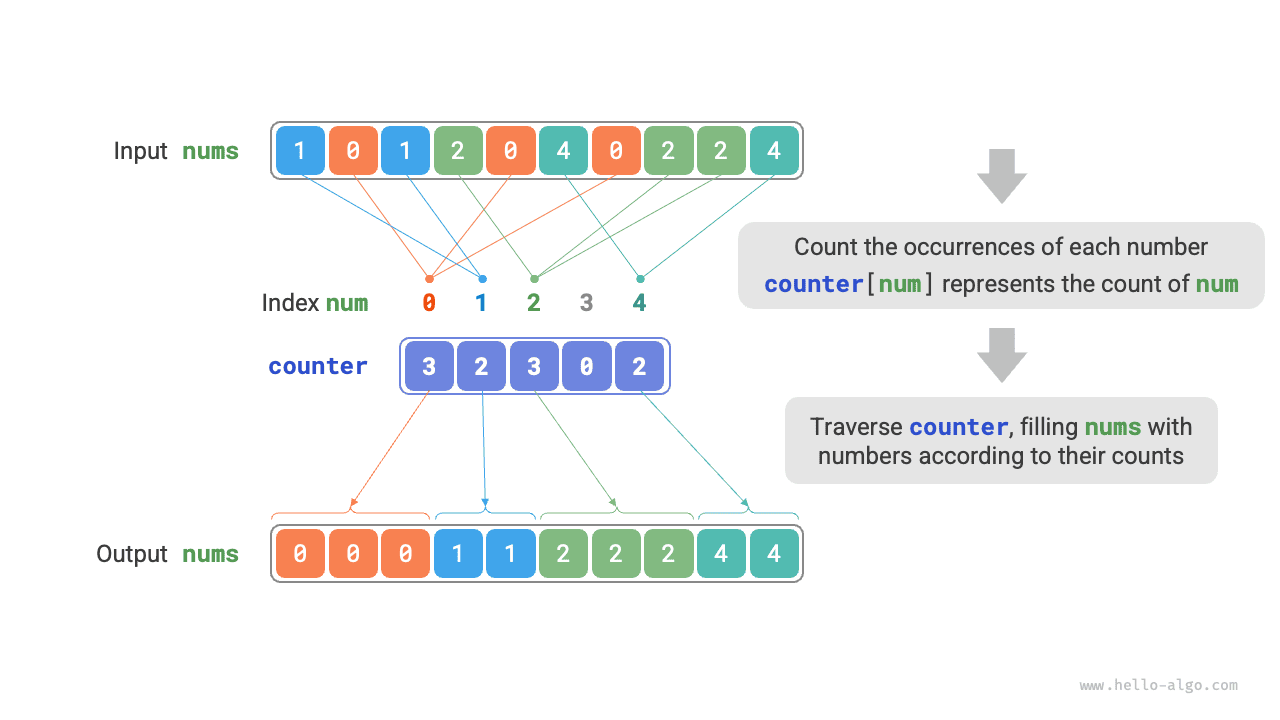
Let's start with a simple example. Given an array nums of length \(n\), where the elements are all "non-negative integers", the overall flow of counting sort is shown in the figure below.
- Traverse the array to find the largest number, denoted as \(m\), and then create an auxiliary array
counterof length \(m + 1\). - Use
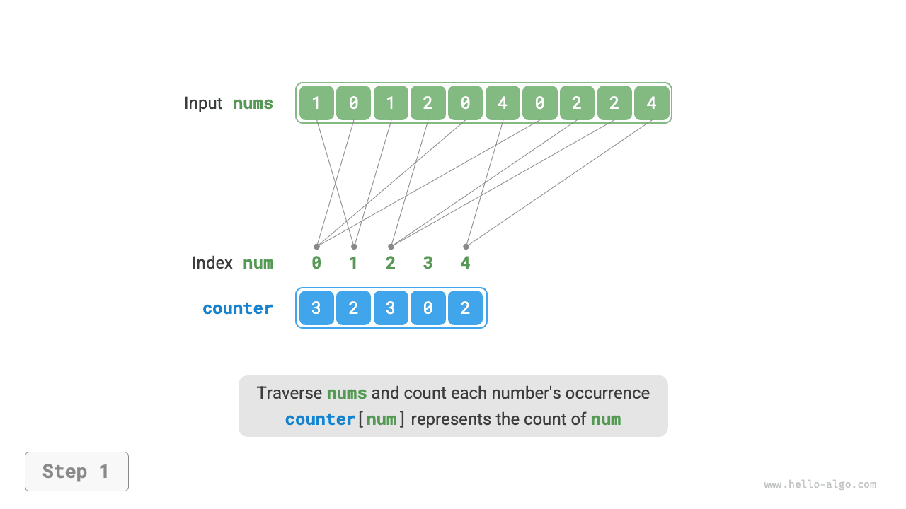
counterto count how many times each number appears innums, wherecounter[num]stores the number of occurrences ofnum. This is simple: traversenums(denote the current number bynum) and incrementcounter[num]by \(1\) each time. - Because the indices of
counterare naturally ordered, the numbers are effectively already sorted. Next, traversecounterand write the numbers back intonumsin ascending order according to their occurrence counts.
The code is as follows:
Connection between counting sort and bucket sort
From the perspective of bucket sort, each index of the counting array counter can be viewed as a bucket, and the counting process can be seen as distributing elements into their corresponding buckets. Essentially, counting sort is a special case of bucket sort for integer data.
Complete Implementation
Observant readers may have noticed that if the input consists of objects, step 3. above no longer works. Suppose the input consists of product objects and we want to sort them by price (a member variable of the class); the above algorithm can only produce the sorted order of the prices themselves.
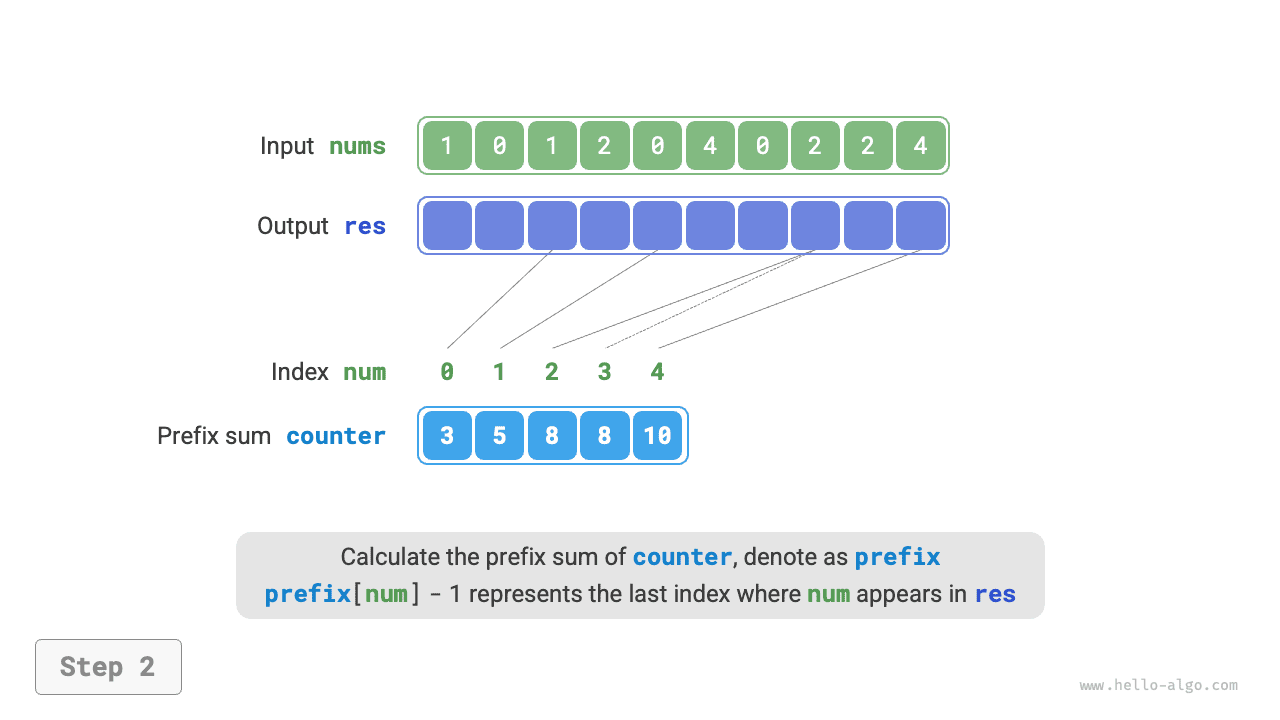
So how can we obtain the sorted order of the original data? We first compute the prefix sums of counter. As the name suggests, the prefix sum at index i, prefix[i], equals the sum of the elements from index 0 through i:
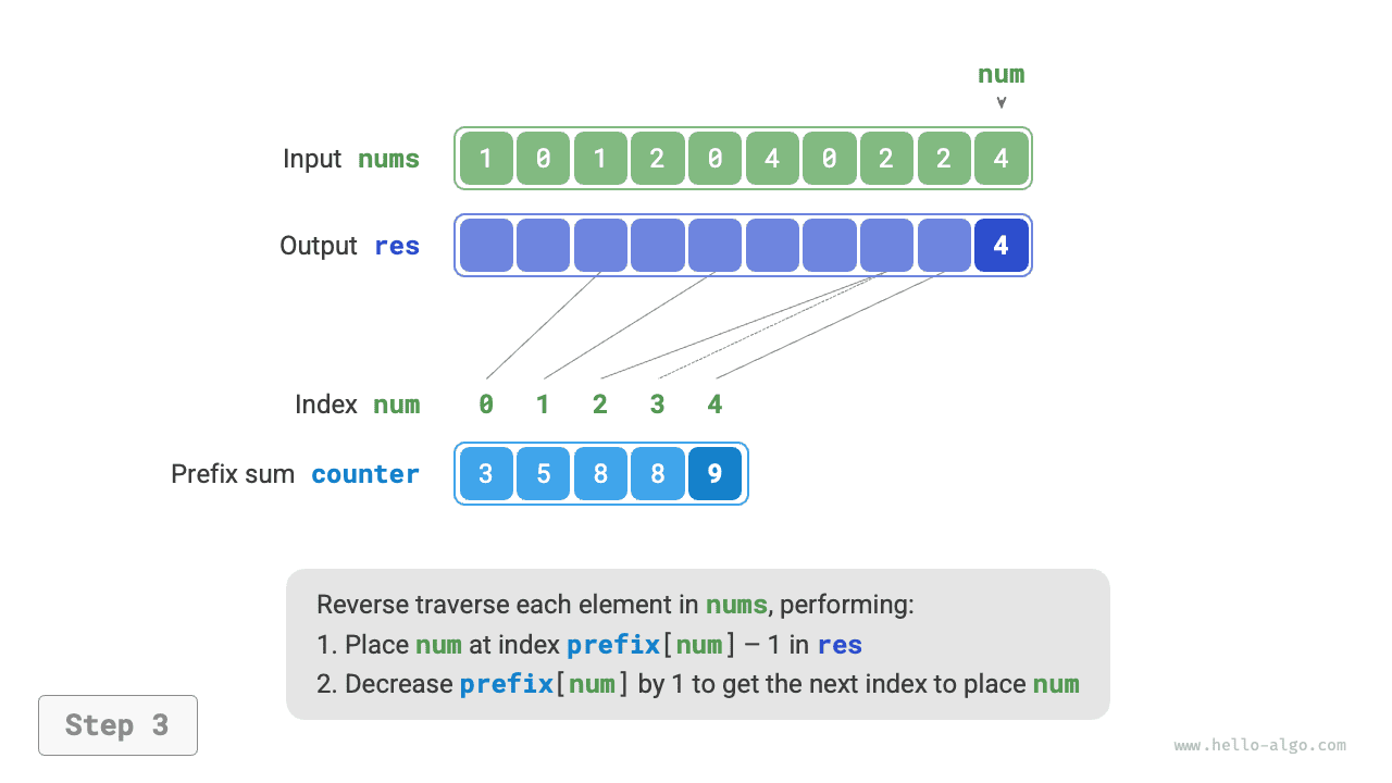
The prefix sum has a clear interpretation: prefix[num] - 1 gives the index of the last occurrence of element num in the result array res. This information is crucial because it tells us where each element should be placed in the result array. Next, we traverse the original array nums in reverse, and for each element num, perform the following two steps.
- Place
numat indexprefix[num] - 1of the arrayres. - Decrease the prefix sum
prefix[num]by \(1\) to get the index for the next placement ofnum.
After the traversal is complete, the array res contains the sorted result, and finally res is used to overwrite the original array nums. The complete counting sort flow is shown in the figure below.
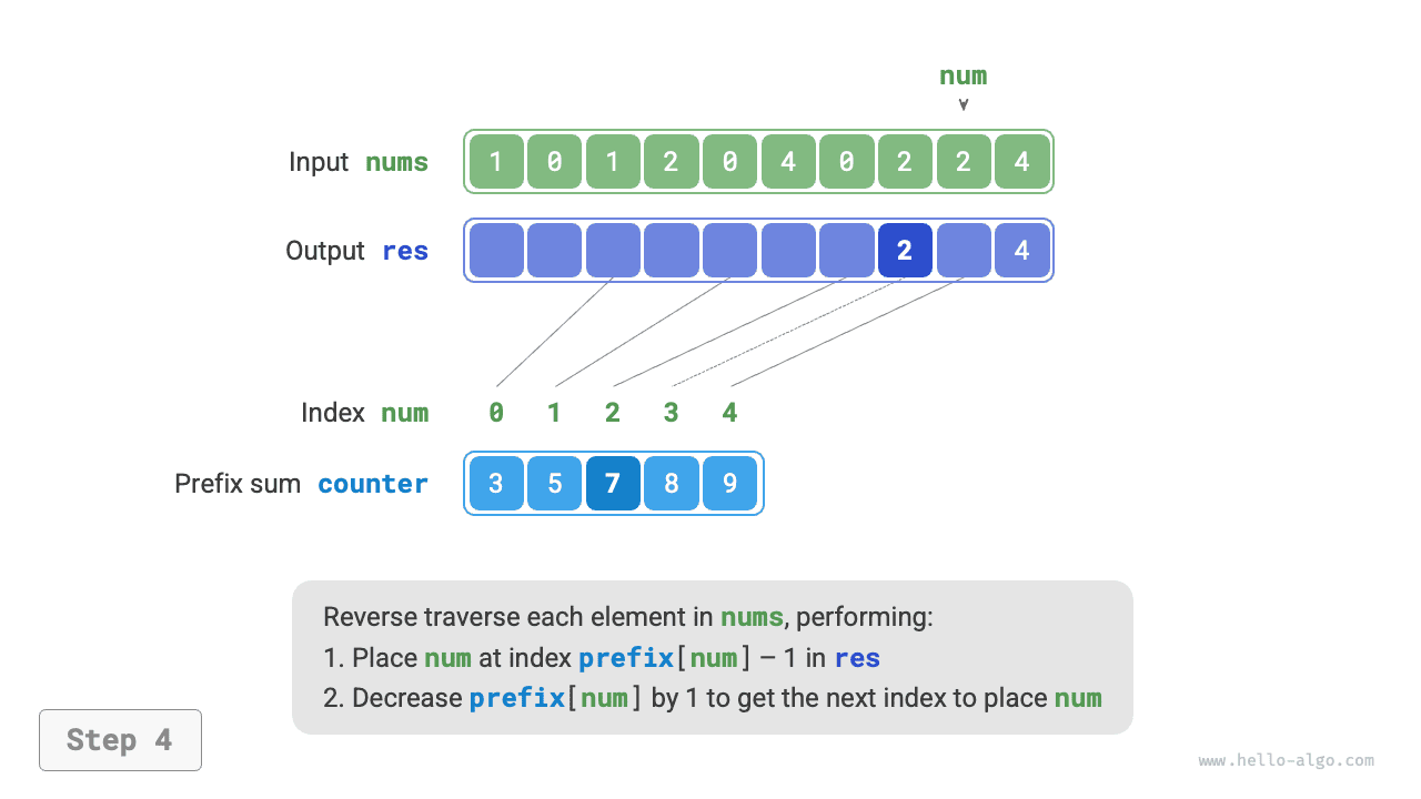
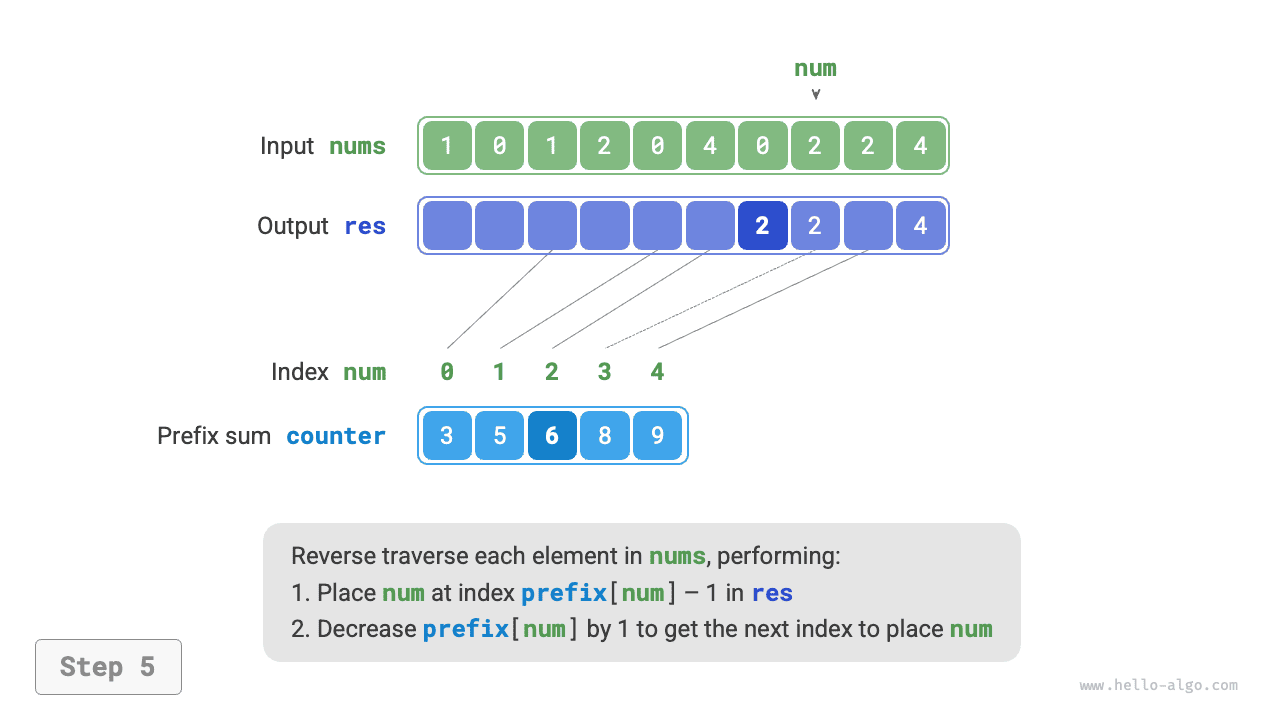
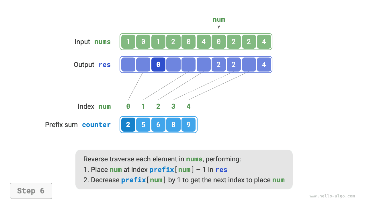
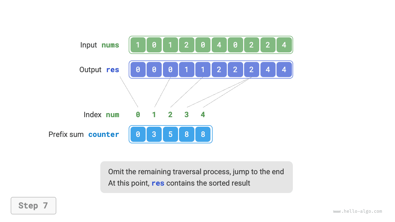
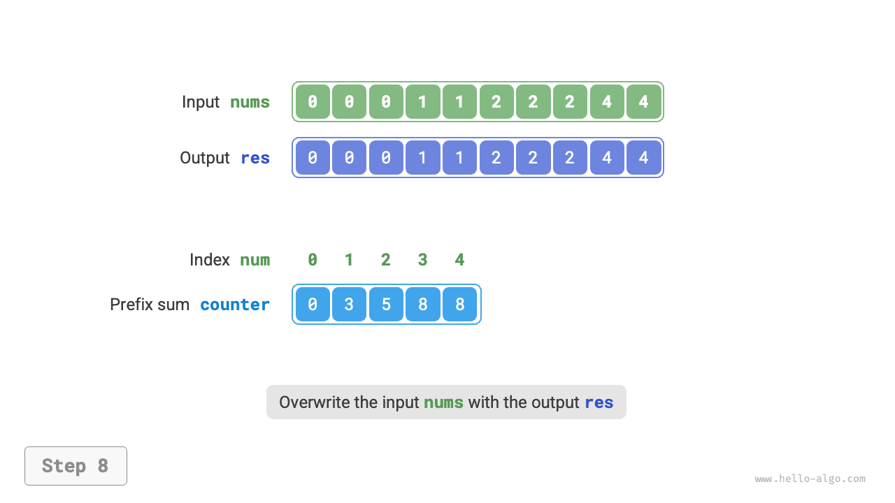
The counting sort implementation is shown below:
Algorithm Characteristics
- Time complexity is \(O(n + m)\), and counting sort is non-adaptive: Traversing
numsandcounterboth takes linear time. In general, when \(n \gg m\), the time complexity approaches \(O(n)\). - Space complexity of \(O(n + m)\), non-in-place sorting: Uses arrays
resandcounterof lengths \(n\) and \(m\) respectively. - Stable sorting: Since elements are filled into
resin a "right-to-left" order, traversingnumsin reverse can avoid changing the relative positions of equal elements, thereby achieving stable sorting. In fact, traversingnumsin forward order can also yield correct sorting results, but the result would be unstable.
Limitations
At this point, you might think counting sort is quite ingenious because it achieves efficient sorting simply by counting occurrences. However, the prerequisites for using counting sort are fairly restrictive.
Counting sort is only applicable to non-negative integers. To apply it to other types of data, you must ensure that they can be converted to non-negative integers without changing the relative ordering of the elements. For example, for an integer array containing negative numbers, you can first add a constant to every number to shift them into the non-negative range, and then shift them back after sorting.
Counting sort is well suited to cases with many elements but a small value range. For example, in the above scenario, \(m\) cannot be too large; otherwise, it consumes too much space. And when \(n \ll m\), counting sort takes \(O(m)\) time, which may be slower than sorting algorithms with \(O(n \log n)\) time complexity.