Quick Sort
Quick sort is an efficient and widely used sorting algorithm based on the divide-and-conquer strategy.
The core operation of quick sort is "sentinel partitioning", whose goal is to select an element as the "pivot", move all elements smaller than the pivot to its left, and move all elements larger than the pivot to its right. Specifically, the process is shown in the figure below.
- Select the leftmost element as the pivot, and initialize two pointers
iandjat the two ends of the array. - Enter a loop. In each round, use
i(j) to find the first element larger (smaller) than the pivot, and then swap the two elements. - Repeat step
2.untiliandjmeet, then swap the pivot into the boundary position between the two sub-arrays.
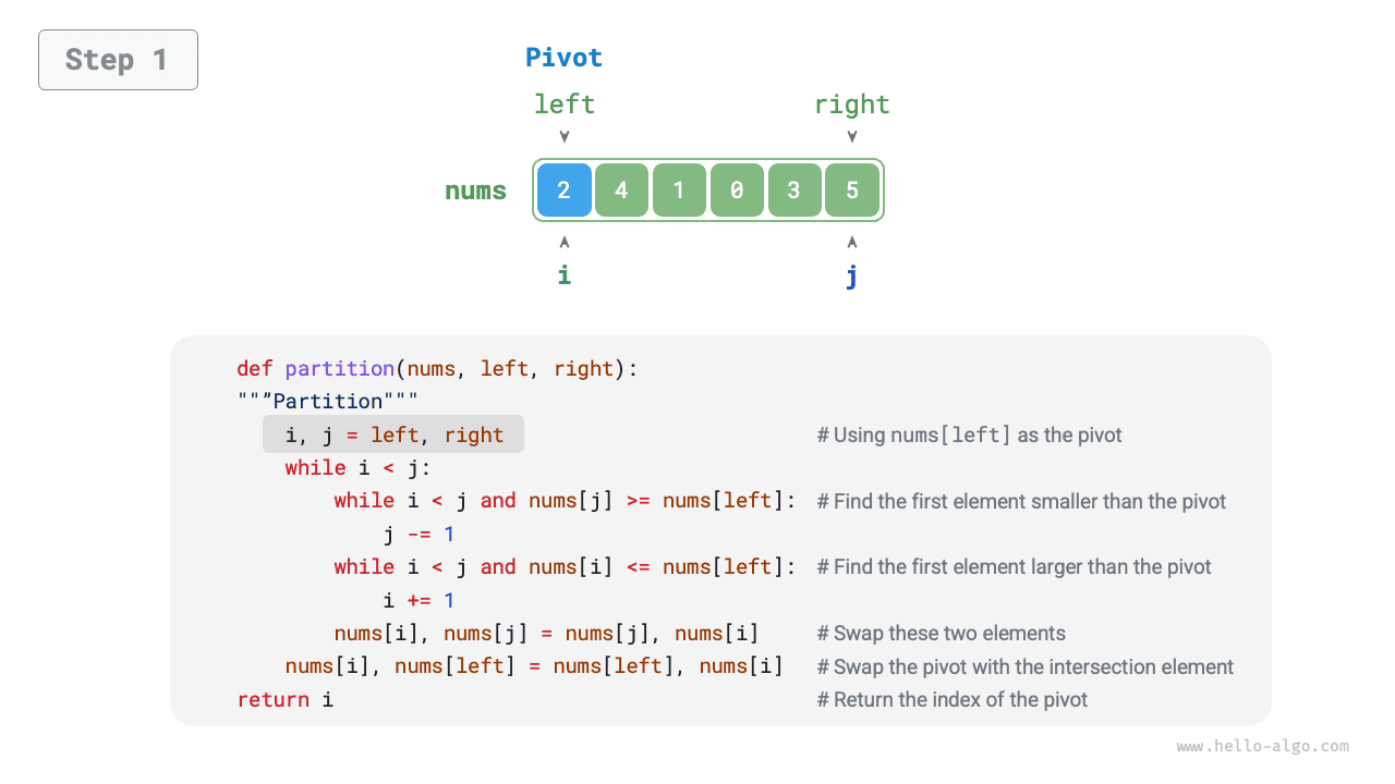
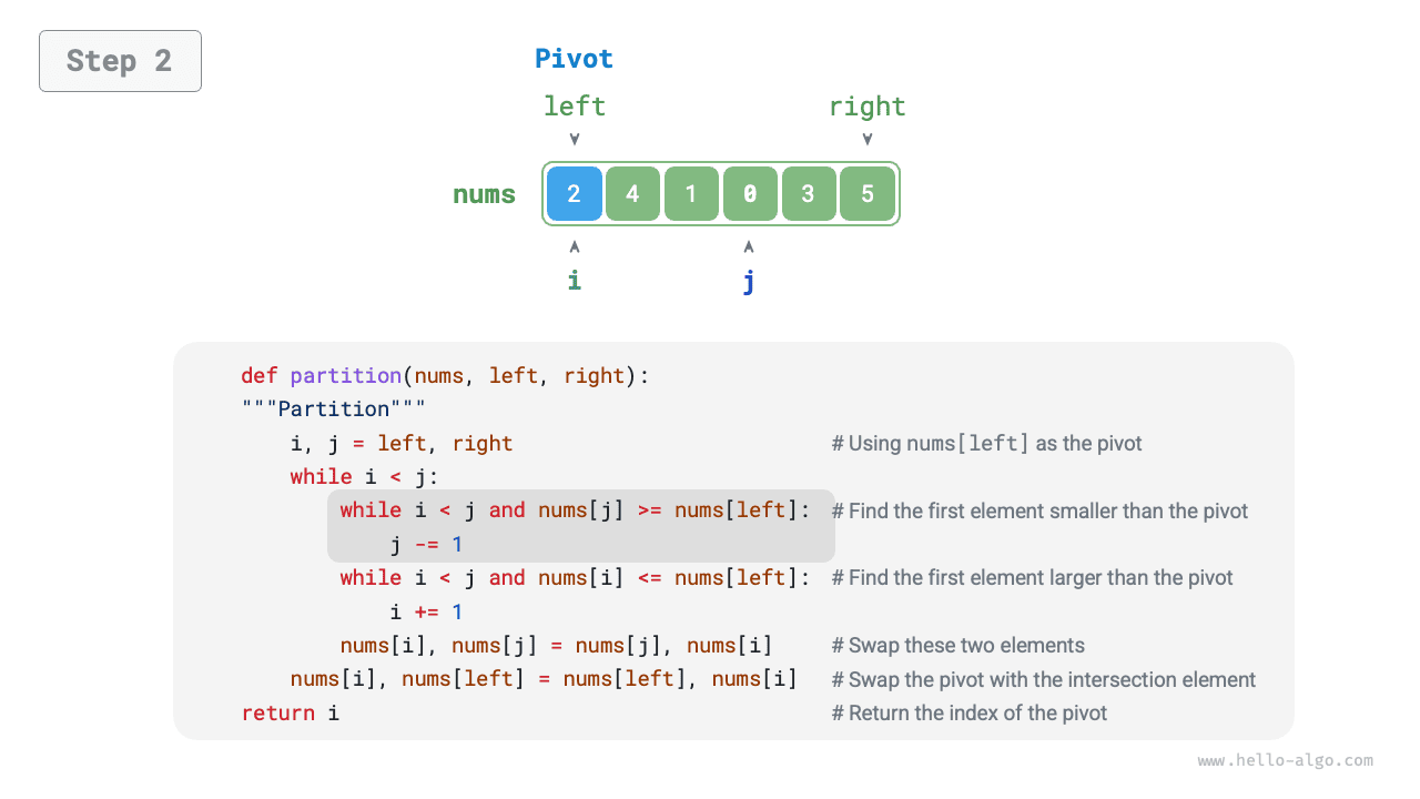
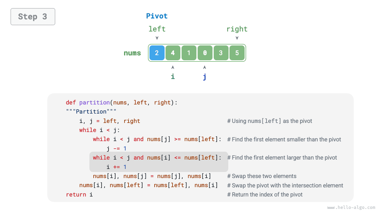
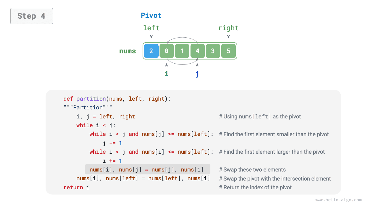
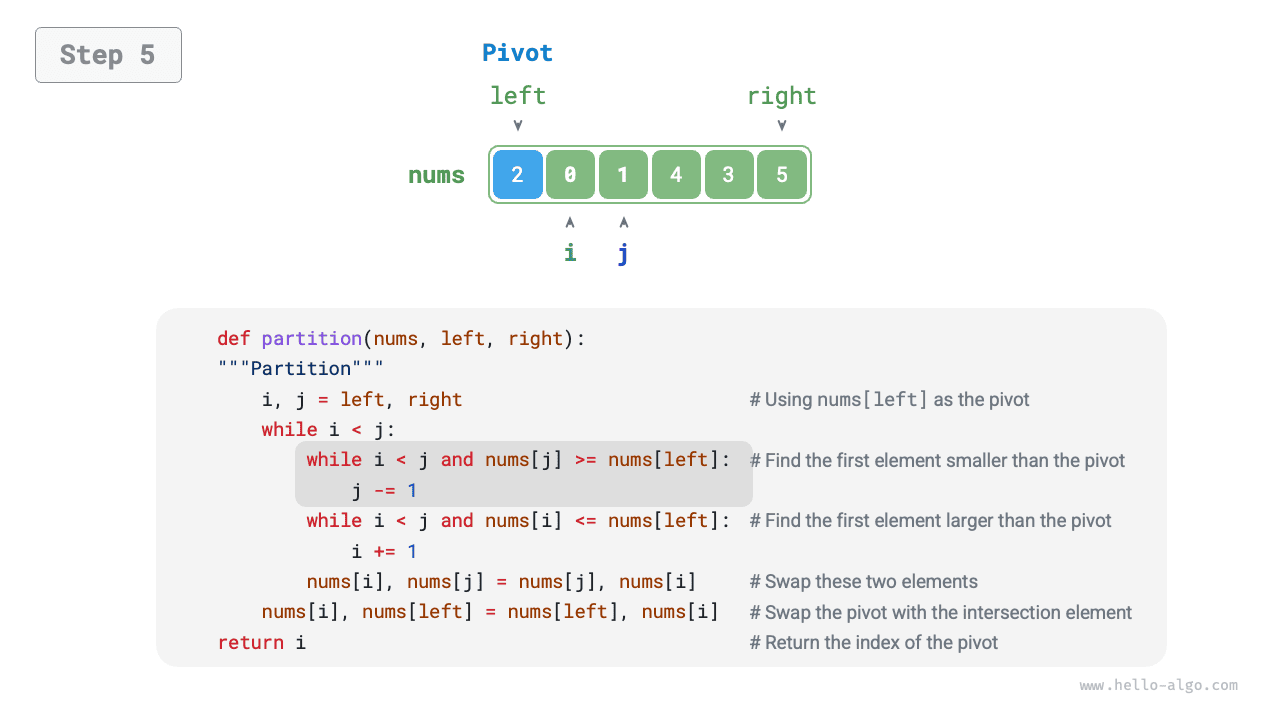
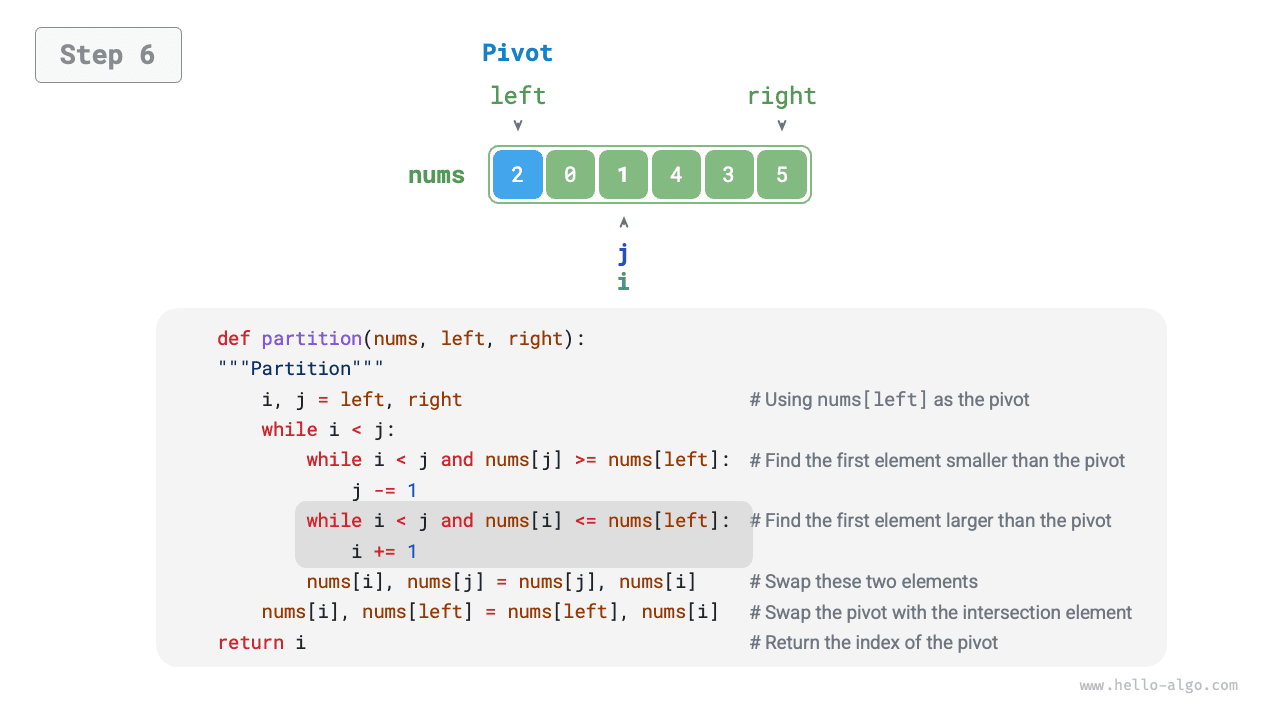
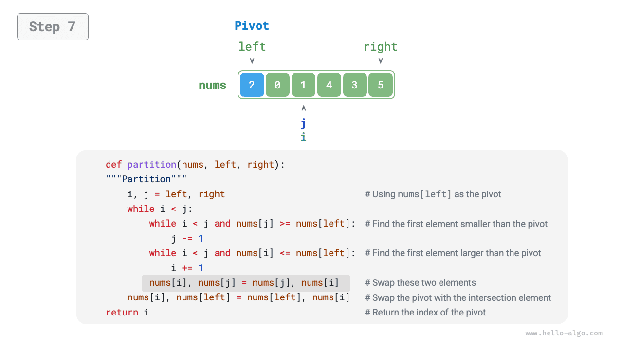
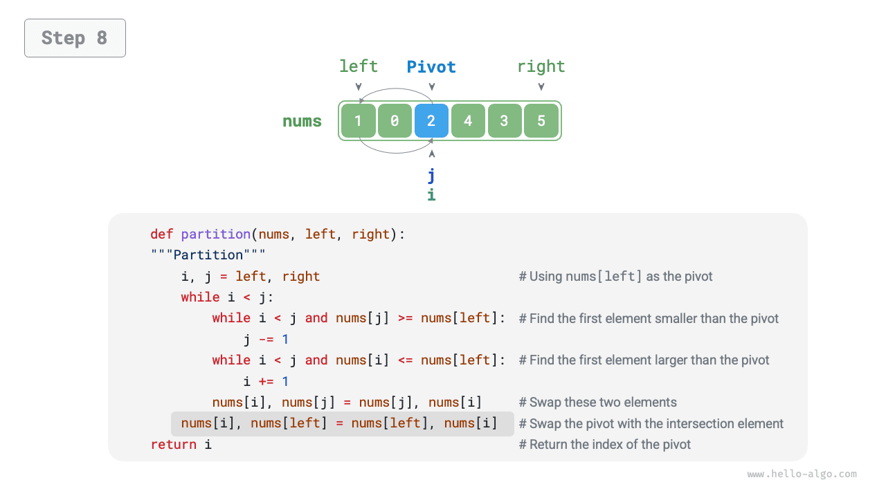
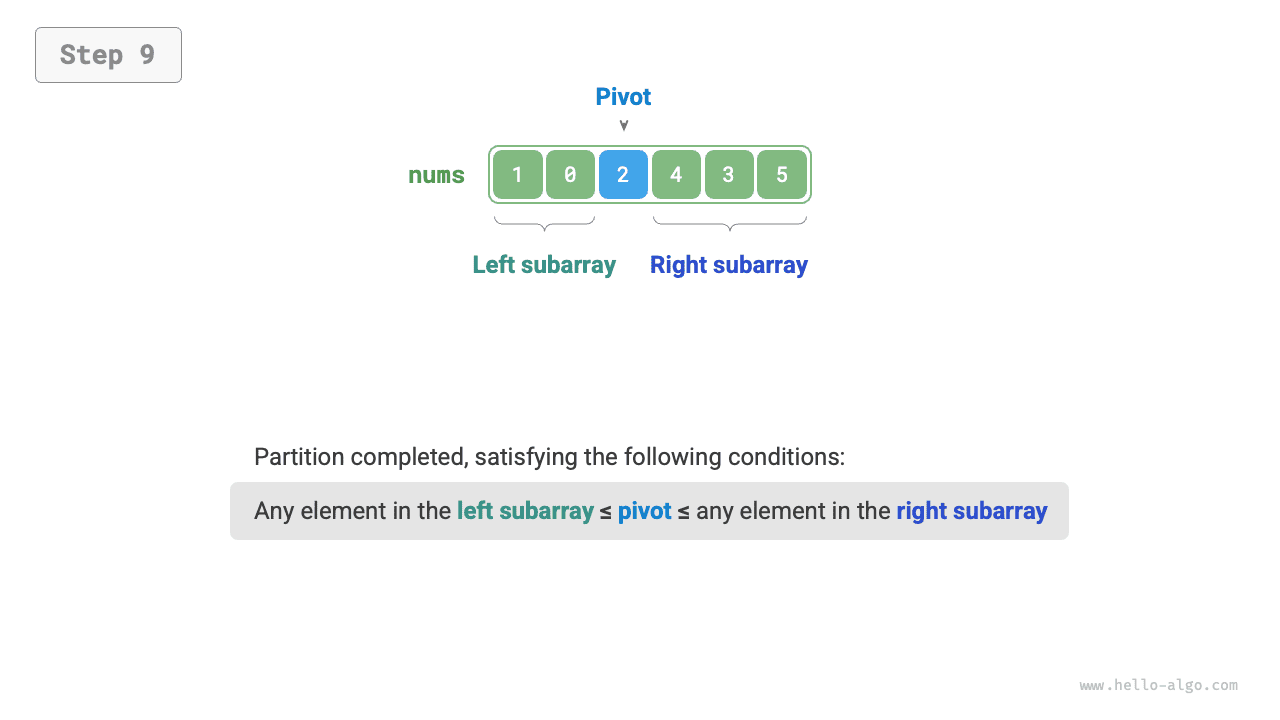
After sentinel partitioning, the original array is divided into three parts: the left sub-array, the pivot, and the right sub-array, such that "any element in the left sub-array \(\leq\) the pivot \(\leq\) any element in the right sub-array". Therefore, we only need to sort the two sub-arrays next.
Divide-and-conquer strategy of quick sort
The essence of sentinel partitioning is to simplify the sorting problem of a longer array into the sorting problems of two shorter arrays.
Algorithm Flow
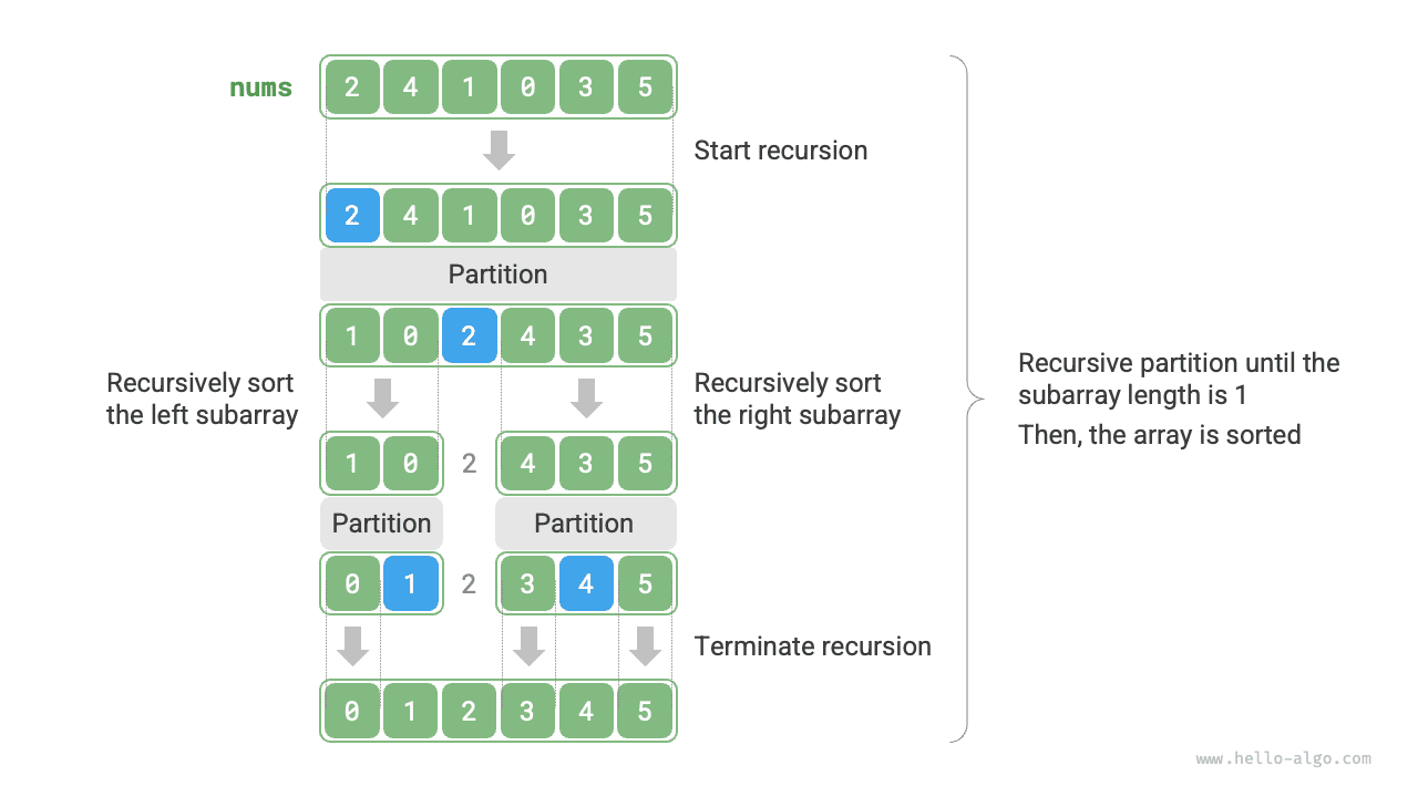
The overall flow of quick sort is shown in the figure below.
- First, perform one "sentinel partitioning" on the original array to obtain the unsorted left sub-array and right sub-array.
- Then, recursively perform "sentinel partitioning" on the left sub-array and right sub-array respectively.
- Continue recursively until the sub-array length is 1, at which point sorting of the entire array is complete.
Algorithm Characteristics
- Time complexity of \(O(n \log n)\), non-adaptive sorting: On average, sentinel partitioning produces \(\log n\) recursive levels, and the total number of loop iterations across each level is \(n\), so the overall time complexity is \(O(n \log n)\). In the worst case, each round of sentinel partitioning splits an array of length \(n\) into sub-arrays of lengths \(0\) and \(n - 1\). The recursion depth then reaches \(n\), with \(n\) loop iterations at each level, yielding an overall time complexity of \(O(n^2)\).
- Space complexity of \(O(n)\), in-place sorting: In the case where the input array is completely reversed, the worst recursive depth reaches \(n\), using \(O(n)\) stack frame space. The sorting operation is performed on the original array without the aid of an additional array.
- Unstable sorting: In the last step of sentinel partitioning, the pivot may be swapped to the right of an equal element.
Why Is Quick Sort Fast
As the name suggests, quick sort has clear efficiency advantages. Although its average time complexity is the same as that of "merge sort" and "heap sort", quick sort is usually faster in practice for the following reasons.
- The worst case is unlikely to occur: Although the worst-case time complexity of quick sort is \(O(n^2)\) and its performance is less predictable than that of merge sort, quick sort runs in \(O(n \log n)\) time in the vast majority of cases.
- High cache efficiency: During sentinel partitioning, the system can load the entire sub-array into cache, so accessing elements is relatively efficient. By contrast, algorithms such as "heap sort" require non-contiguous access to elements and therefore do not enjoy this advantage.
- Small constant factors: Among the three algorithms above, quick sort performs the fewest comparisons, assignments, and swaps in total. This is similar to why "insertion sort" is faster than "bubble sort".
Pivot Optimization
Quick sort can become less time-efficient for certain inputs. Consider an extreme example in which the input array is in completely descending order. Because we choose the leftmost element as the pivot, once sentinel partitioning is complete, the pivot is swapped to the far right of the array, leaving a left sub-array of length \(n - 1\) and a right sub-array of length \(0\). If this continues recursively, each round of sentinel partitioning produces one sub-array of length \(0\), the divide-and-conquer strategy breaks down, and quick sort degenerates into an approximation of "bubble sort".
To reduce the chance of this happening, we can optimize the pivot selection strategy used in sentinel partitioning. For example, we can choose a pivot at random. However, if we are unlucky and repeatedly pick poor pivots, performance can still be unsatisfactory.
It should be noted that programming languages usually generate "pseudo-random numbers". If we construct a specific test case against a pseudo-random sequence, quick sort can still suffer degraded performance.
To improve further, we can choose three candidate elements from the array, usually the first, last, and middle elements, and use the median of the three as the pivot. This greatly increases the chance that the pivot is "neither too small nor too large". We can also choose more candidate elements to further improve the robustness of the algorithm. With this method, the probability that the time complexity degrades to \(O(n^2)\) is significantly reduced.
Example code is as follows:
Recursive Depth Optimization
Quick sort may also use more space for certain inputs. Consider a fully sorted input array. Let the length of the current sub-array in the recursion be \(m\). Each round of sentinel partitioning produces a left sub-array of length \(0\) and a right sub-array of length \(m - 1\), which means each recursive call reduces the problem size by only one element. The recursion tree can therefore reach a height of \(n - 1\), requiring \(O(n)\) stack-frame space.
To prevent stack frames from accumulating, we can compare the lengths of the two sub-arrays after each round of sentinel partitioning, and recurse only on the shorter one. Because the shorter sub-array has length at most \(n / 2\), this method ensures that the recursion depth does not exceed \(\log n\), reducing the worst-case space complexity to \(O(\log n)\). The code is shown below: