Insertion Sort
Insertion sort is a simple sorting algorithm that works very similarly to the process of manually sorting a deck of cards.
Specifically, we select a base element from the unsorted portion, compare it one by one with the elements in the sorted portion to its left, and insert it into the correct position.
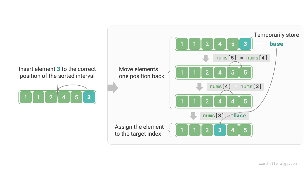
The figure below illustrates how an element is inserted into an array. Let the base element be base. We need to shift all elements between the target index and base one position to the right, and then assign base to the target index.
Algorithm Flow
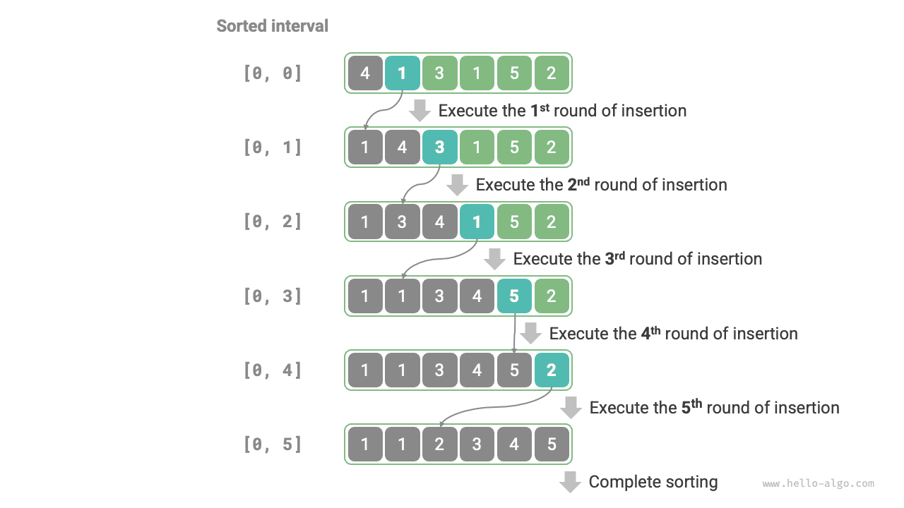
The overall flow of insertion sort is shown in the figure below.
- Initially, the first element of the array is already sorted.
- Select the second element of the array as
base, and after inserting it into the correct position, the first 2 elements of the array are sorted. - Select the third element as
base, and after inserting it into the correct position, the first 3 elements of the array are sorted. - And so on. In the last round, select the last element as
base, and after inserting it into the correct position, all elements are sorted.
Example code is as follows:
Algorithm Characteristics
- Time complexity of \(O(n^2)\), adaptive sorting: In the worst case, the insertion operations require \(n - 1\), \(n-2\), \(\dots\), \(2\), and \(1\) iterations, respectively, summing to \((n - 1) n / 2\), so the time complexity is \(O(n^2)\). When the data is already sorted, each insertion operation terminates early. When the input array is completely sorted, insertion sort achieves its best-case time complexity of \(O(n)\).
- Space complexity of \(O(1)\), in-place sorting: Pointers \(i\) and \(j\) use a constant amount of extra space.
- Stable sorting: During insertion, we place elements to the right of equal elements, so their relative order is unchanged.
Advantages of Insertion Sort
The time complexity of insertion sort is \(O(n^2)\), while the time complexity of quick sort, which we will learn about next, is \(O(n \log n)\). Although insertion sort has a higher time complexity, it is usually faster on small datasets.
This conclusion is similar to the one about when linear search and binary search are applicable. Algorithms such as quick sort, with \(O(n \log n)\) complexity, are divide-and-conquer sorting algorithms and often involve more primitive operations. When the dataset is small, the values of \(n^2\) and \(n \log n\) are relatively close, so asymptotic complexity does not dominate; instead, the number of primitive operations per round becomes the deciding factor.
In fact, the built-in sorting functions of many programming languages (such as Java) use insertion sort. The general idea is: for large arrays, use divide-and-conquer sorting algorithms such as quick sort; for short arrays, use insertion sort directly.
Although bubble sort, selection sort, and insertion sort all have a time complexity of \(O(n^2)\), in actual situations, insertion sort is used significantly more frequently than bubble sort and selection sort, mainly for the following reasons.
- Bubble sort is implemented through element swaps, which require a temporary variable and involve 3 primitive operations; insertion sort is implemented through element assignment and requires only 1 primitive operation. Therefore, bubble sort usually has higher computational overhead than insertion sort.
- Selection sort has a time complexity of \(O(n^2)\) in any case. If given a set of partially ordered data, insertion sort is usually more efficient than selection sort.
- Selection sort is unstable and cannot be applied to multi-level sorting.